Improving histogram usability for Prometheus and Grafana

It looks like histogram support is great in Prometheus ecosystem:

• Prometheus client libraries provide Histogram metrics.
• Prometheus provides histogram_quantile function for calculating quantiles over histogram buckets.
• Grafana supports visualizing Prometheus histogram buckets via Heatmap panel.

But why Prometheus users continue complaining about issues in histograms? Let’s look at the most annoying issues.

Issue #1: metric range isn’t covered well by the defined histogram buckets

Suppose you decided covering response size with Prometheus histograms and defined the following histogram according to docs:

h := prometheus.NewHistogram(prometheus.HistogramOpts{
    Name:    "response_size_bytes",
    Help:    "The size of the response",
    Buckets: prometheus.LinearBuckets(100, 100, 3),
})

This histogram has 4 buckets with the following response size ranges (aka le label value):

• (0…100] aka le=”100"
• (0…200] aka le=”200"
• (0…300] aka le=”300"
• (0…+Inf] aka le=”+Inf”

After some time you noticed that big number of response sizes fit the first bucket, i.e. they have sizes smaller or equal to 100 bytes. If you want determining response sizes on the (0…100] range more precisely, you have to adjust Buckets value in the source code above to something like the following:

Buckets: [10, 20, 40, 80, 100, 200, 300]

Now you have 5 buckets on the range (0…100], so you can determine response size more precisely. You are happy! But the response size can grow over time like any page size on the Internet. When the majority of response sizes become greater than 300 bytes, your buckets become useless. You add another portion of buckets to the histogram. Then repeat it every few months until the number of buckets grows to hundreds and become unmaintainable mess.

Issue #2: too many buckets and high cardinality

The number of per-histogram buckets can rapidly grow as you could see from the previous chapter. Each histogram bucket is stored as a separate time series in Prometheus. This means that the number of unique time series can quickly go out of control, which will result in high cardinality issues:

• High RAM usage, since TSDB usually keeps meta-information about each time series in RAM. See, for example, Thanos Store Gateway high RAM usage and OOMs.
• High disk space usage, since each time series data requires additional disk space. See, for example, high disk space usage in Thanos Compactor.
• Slower performance for inserts, since TSDB must perform more bookkeeping when storing samples for higher number of active time series.
• Slower performance for selects, since each query would process more time series for higher number of buckets before returning the result.

While certain TSDB solutions can keep better with high cardinality (see this and this post), all of them still suffer from the issues mentioned above.

Issue #3: incompatible bucket ranges

Suppose your app has two histograms:

• Response time for public pages — response_time_seconds{zone=”public”} with the following buckets: [0.1, 0.2, 0.3, 0.4, 0.5], since it is expected that publicly-facing pages must be returned in less than 0.5 seconds.
• Response time for admin pages — response_time_seconds{zone=”admin”} with the following buckets: [0.5, 1.0, 1.5, 2.0, 5.0], since admins aren’t so sensitive to response times comparing to public page visitors.

You decided calculating summary quantile over public pages and admin pages with the following PromQL query according to docs:

histogram_quantile(0.95,
    sum(rate(
        response_time_seconds_bucket{zone=~"public|admin"}[5m]
    )) by (le)
)

But the query returns garbage because response times for public and admin pages have different set of buckets :(

The solution — VictoriaMetrics histogram

We at VictoriaMetrics decided fixing these issues, went to drawing board, designed human-friendly easy-to-use Histogram and added it to the lightweight client library for exposing Prometheus-compatible metrics — github.com/VictoriaMetrics/metrics. The Histogram just works:

• There is no need in thinking about bucket ranges and the number of buckets per histogram, since buckets are created on demand.
• There is no need in worrying about high cardinality, since only buckets with non-zero values are exposed to Prometheus. Usually real-world values are located on quite small range, so they are covered by small number of histogram buckets.
• There is no need in re-configuring buckets over time, since bucket configuration is static. This allows performing cross-histogram calculations. For instance, the following query should work as expected in VictoriaMetrics starting from release v1.30.0:

histogram_quantile(0.95,
    sum(rate(
        response_time_seconds_bucket{zone=~"public|admin"}[5m]
    )) by (vmrange)
)

Unfortunately this query doesn’t work in Prometheus, since it is unaware of VictoriaMetrics histograms yet. So set up VictoriaMetrics as a remote storage for Prometheus according to these simple docs and enjoy the power of user-friendly histograms. Or just use vmagent for sending data to VictoriaMetrics.

VictoriaMetrics histogram internals

Histogram covers values in the following range: [10-⁹…10¹⁸]. This includes:

• Times from nanoseconds to billions of years.
• Sizes from 0 bytes to 2⁶⁰ bytes.

The Histogram splits each (10^n...10^(n+1)] range into 18 log-based buckets with 10^(1/18)=1.136 multiplier:

(1.0*10^n…1.136*10^n], (1.136*10^n…1.292*10^n], … (8.799*10^n…1.0*10^(n+1)]

This gives 13.6% worst-case precision error, which is enough for most practical cases. It is easy to start using Histogram in your apps:

// create histogram for response sizes
var responseSize = metrics.NewHistogram("response_size_bytes")
...
func sendResponse(w io.Writer, response []byte) {
    w.Write(response)
    // Register the response size in histogram
    responseSize.Update(float64(len(response)))
}

See usage docs for github.com/VictoriaMetrics/metrics here.

Bonus: using the power of heatmaps in Grafana

Grafana is able to build pretty heatmaps from Prometheus-style histogram buckets, but it is unaware of VictoriaMetrics-style histograms. So the following PromQL extension functions are provided in VictoriaMetrics starting from v1.30.0:

• prometheus_buckets() function for converting VictoriaMetrics histogram buckets to Promethues-compatible buckets with le labels, which can be built with Grafana heatmaps:

prometheus_buckets(
    sum(rate(
        vm_http_request_duration_seconds_bucket
    )) by (vmrange)
)

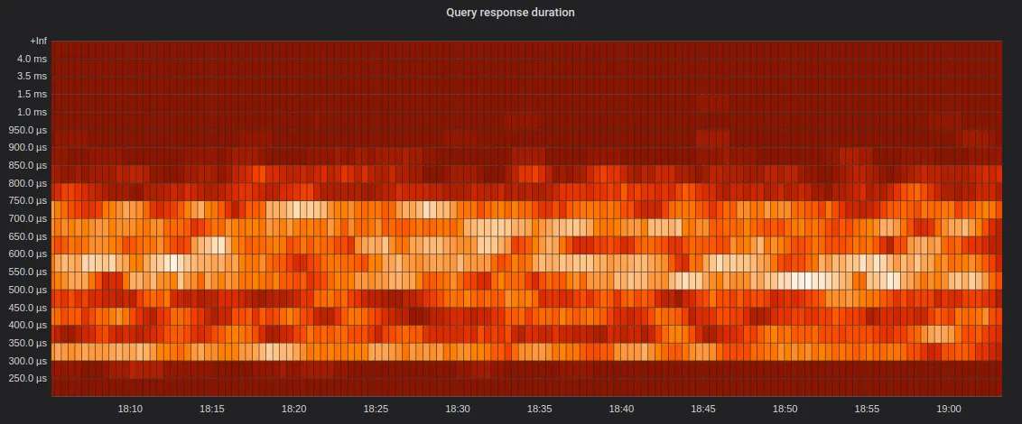
Grafana would build the following heatmap for this query:

It is easy to notice from the heatmap that the majority of requests are executed in 0.35ms — 0.8ms.

• buckets_limit() function, which limits the number of buckets per metric. This function may be useful for building heatmaps from big number of buckets. The heatmap may be difficult to read if the number of buckets is too big. Just wrap the result into buckets_limit(N, ...) in order to limit the number of buckets to N. For example, the following query would return up to 10 resulting buckets for heatmap in Grafana:

buckets_limit(10, sum(rate(vm_http_request_duration_seconds_bucket)) by (vmrange))

• histogram() aggregate function for building Prometheus-style histogram buckets from a set of time series. For example, the following query:

histogram(process_resident_memory_bytes)

Would return the following graph over a fleet of Go apps, which export metrics in Prometheus format via github.com/VictoriaMetrics/metrics library:

histogram(process_resident_memory_bytes)

As you can see from the graph, the majority of Go apps in the fleet use 15–20MB of RAM, while there are apps in the fleet that use 150-200MB of RAM. The heatmap provides much better visual information comparing to simple lines, especially when building graphs over thousands of time series. Just compare the above heatmap to the usual graph below for the same time series:

process_resident_memory_bytes

Conclusion

Histograms in Prometheus are tricky to use. VictoriaMetrics simplifies this with Histogram from github.com/VictoriaMetrics/metrics library and new functions added to MetricsQL starting from v1.30.0 release. Give it a try and forget about issues with old-style Prometheus histograms :)

Update: now VictoriaMetrics provides additional functions, which could be useful when working with histograms:

• histogram_over_time(m[d]) for calculating histogram for gauge values m over the given time window d.
• histogram_share(le, buckets) for calculating service level indicator (aka SLI / SLO). It returns the share (phi) for bucket values that don’t exceed the given threshold le. This is the inverse of histogram_quantile(phi, buckets).
• share_le_over_time(m[d], le) for calculating SLI / SLO / SLA for gauge values m over the given time window d, that don’t exceed the given threshold le.

See the full list of additional functions in MetricsQL.

P.S. Join our Slack channel and ask additional questions about VictoriaMetrics histograms.